This article has been posted for discussion at Judith Curry’s “Climate Etc.”
On determination of tropical feedbacks
Abstract
Satellite data for the period surrounding the Mt Pinatubo eruption in 1991 provide a means of estimating the scale of the volcanic forcing in the tropics. A simple relaxation model is used to examine how temporal evolution of the climate response will differ from the that of the radiative forcing. Taking this difference into account is essential for proper detection and attribution of the relevant physical processes. Estimations are derived for both the forcing and time-constant of the climate response. These are found to support values derived in earlier studies which vary considerably from those of current climate models. The implications of these differences in inferring climate sensitivity are discussed. The study reveals the importance of secondary effects of major eruptions pointing to a persistent warming effect in the decade following the 1991 eruption.
The inadequacy of the traditional application of linear regression to climate data is highlighted, showing how this will typically lead to erroneous results and thus the likelihood of false attribution.
The implications of this false attribution to the post-2000 divergence between climate models and observations is discussed.
Keywords: climate; sensitivity; tropical feedback; global warming; climate change; Mount Pinatubo; volcanism; GCM; model divergence; stratosphere; ozone; multivariate; regression; ERBE; AOD ;
Introduction
For the period surrounding the eruption of Mount Pinatubo in the Philippines in June 1991, there are detailed satellite data for both the top-of-atmosphere ( TOA ) radiation budget and atmospheric optical depth ( AOD ) that can be used to derive the changes in radiation entering the climate system during that period. Analysis of these radiation measurements allows an assessment of the system response to changes in the radiation budget. The Mt. Pinatubo eruption provides a particularly useful natural experiment, since the spread of the effects were centred in the tropics and dispersed fairly evenly between the hemispheres. [1] fig.6 ( This meta-study provides a lot of detail about the composition and dispersal of the aerosol cloud.)
The present study investigates the tropical climate response in the years following the eruption. It is found that a simple relaxation response, driven by volcanic radiative ‘forcing’, provides a close match with the variations in TOA energy budget. The derived scaling factor to convert AOD into radiative flux, supports earlier estimations [2] based on observations from the 1982 El Chichon eruption. These observationally derived values of the strength of the radiative disturbance caused by major stratospheric eruptions are considerably greater than those currently used as input parameters for general circulation climate models (GCMs). This has important implications for estimations of climate sensitivity to radiative ‘forcings’ and attribution of the various internal and external drivers of the climate system.
Method
Changes in net TOA radiative flux, measured by satellite, were compared to volcanic forcing estimated from measurements of atmospheric optical depth. Regional optical depth data, with monthly resolution, are available in latitude bands for four height ranges between 15 and 35 km [DS1] and these values were averaged from 20S to 20N to provide a monthly mean time series for the tropics. Since optical depth is a logarithmic scale, the values for the four height bands were added at each geographic location. Lacis et al [2] suggest that aerosol radiative forcing can be approximated by a linear scaling factor of AOD over the range of values concerned. This is the approach usually adopted in IPCC reviewed assessments and is used here. As a result the vertical summations are averaged across the tropical latitude range for comparison with radiation data.
Tropical TOA net radiation flux is provided by Earth Radiation Budget Experiment ( ERBE ) [DS2].
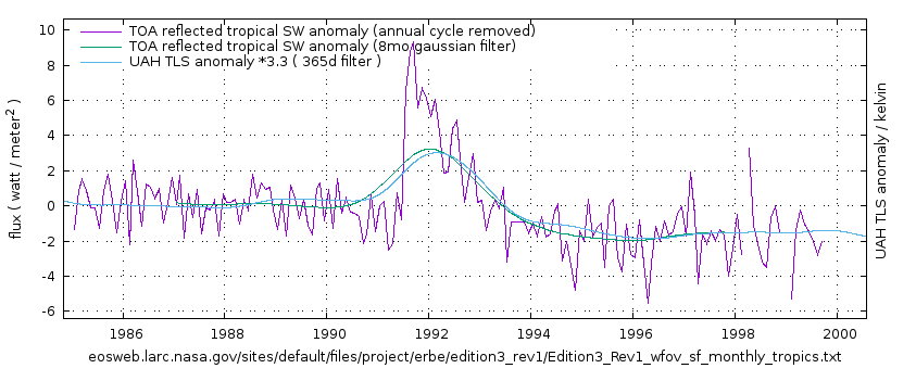
One notable effect of the eruption of Mt Pinatubo on tropical energy balance is a variation in the nature of the annual cycle, as see by subtracting the pre-eruption, mean annual variation. As well as the annual cycle due to the eccentricity of the Earth’s orbit which peaks at perihelion around 4th January, the sun passes over the tropics twice per year and the mean annual cycle in the tropics shows two peaks: one in March the other in Aug/Sept, with a minimum in June and a lesser dip in January. Following the eruption, the residual variability also shows a six monthly cycle. The semi-annual variability changed and only returned to similar levels after the 1998 El Nino.

Figure 1 showing the variability of the annual cycle in net TOA radiation flux in tropics. (Click to enlarge)
It follows that using a single period as the basis for the anomaly leaves significant annual residuals. To minimise the residual, three different periods each a multiple of 12 months were used to remove the annual variations: pre-1991; 1992-1995; post 1995.
The three resultant anomaly series were combined, ensuring the difference in the means of each period were respected. The mean of the earlier, pre-eruption annual cycles was taken as the zero reference for the whole series. There is a clearly repetitive variation during the pre-eruption period that produces a significant downward trend starting 18 months before the Mt. Pinatubo event. Since it may be important not to confound this with the variation due to the volcanic aerosols, it was characterised by fitting a simple cosine function. This was subtracted from the fitting period. Though the degree to which this can be reasonably assumed to continue is speculative, it seems some account needs to be taken of this pre-existing variability. The effect this has on the result of the analysis is assessed.
The break of four months in the ERBE data at the end of 1993 was filled with the anomaly mean for the period to provide a continuous series.

Figure 2 showing ERBE tropical TOA flux adaptive anomaly. (Click to enlarge)

Figure 2b showing ERBE tropical TOA flux adaptive anomaly with pre-eruption cyclic variability subtracted. (Click to enlarge)
Since the TOA flux represents the net sum of all “forcings” and the climate response, the difference between the volcanic forcing and the anomaly in the energy budget can be interpreted as the climate response to the radiative perturbation caused by the volcanic aerosols. This involves some approximations. Firstly, since the data is restricted to the tropical regions, the vertical energy budget does not fully account for energy entering and leaving the region. There is a persistent flow of energy out of the tropics both via ocean currents and atmospheric circulation. Variations in wind driven ocean currents and atmospheric circulation may be part of any climate feedback reaction.
Secondly, taking the difference between TOA flux and the calculated aerosol forcing at the top of the troposphere to represent the top of troposphere energy budget assumes negligible energy is accumulated or lost internally to the upper atmosphere. Although there is noticeable change in stratospheric temperature as a result of the eruption, the heat capacity of the rarefied upper atmosphere means this is negligible in this context.
 Figure 3 showing changes in lower stratosphere temperature due to volcanism. (Click to enlarge)
A detailed study on the atmospheric physics and radiative effects of stratospheric aerosols by Lacis, Hansen & Sato [2] suggested that radiative forcing at the tropopause can be estimated by multiplying optical depth by a factor of 30 W / m2.
This value provides a reasonably close match to the initial change in ERBE TOA flux. However, later studies[3], [4] , attempting to reconcile climate model output with the surface temperature record have reduced the estimated magnitude of the effect stratospheric aerosols. With the latter adjustments, the initial effect on net TOA flux is notably greater than the calculated forcing, which is problematic; especially since Lacis et al reported that the initial cooling may be masked by the warming effect of larger particles ( > 1µm ). Indeed, in order for the calculated aerosol forcing to be as large as the initial changes in TOA flux, without invoking negative feedbacks, it is necessary to use a scaling of around 40 W/m2. A comparison of these values is shown in figure 4.
What is significant is that from just a few months after the eruption, the disturbance in TOA flux is consistently less than the volcanic forcing. This is evidence of a strong negative feedback in the tropical climate system acting to counter the volcanic perturbation. Just over a year after the eruption, it has fully corrected the radiation imbalance despite the disturbance in AOD still being at about 50% of its peak value. The net TOA reaction then remains positive until the “super” El Nino of 1998. This is still the case with reduced forcing values of Hansen et al as can also be seen in figure 4.

Figure 4 comparing volcanic of net TOA flux to various estimations aerosol forcing. ( Click to enlarge )
The fact that the climate is dominated by negative feedbacks is not controversial since this is a pre-requisite for overall system stability. The main stabilising feedback is the Planck response ( about 3.3 W/m2/K at typical ambient temperatures ). Other feedbacks will increase or decrease the net feedback around this base-line value. Where IPCC reports refer to net feedbacks being positive or negative, it is relative to this value. The true net feedback will always be negative.
It is clear that the climate system takes some time to respond to initial atmospheric changes. It has been pointed out that to correctly compare changes in radiative input to surface temperatures some kind of lag-correlation analysis is required : Spencer & Braswell 2011[5], Lindzen & Choi 2011[6] Trenberth et al 2010 [7]. All three show that correlation peaks with the temperature anomaly leading the change in radiation by about three months.

Figure 5 showing climate feedback response to Mt Pinatubo eruption. Volcanic forcing per Lacis et al. ( Click to enlarge )
After a few months, negative feedbacks begin to have a notable impact and the TOA flux anomaly declines more rapidly than the reduction in AOD. It is quickly apparent that a simple, fixed temporal lag is not an appropriate way to compare the aerosol forcing to its effects on the climate system.
The simplest physical response of a system to a disturbance would be a linear relaxation model, or “regression to the equilibrium”, where for a deviation of a variable X from its equilibrium value, there is a restoring action that is proportional to the magnitude of that deviation. The more it is out of equilibrium the quicker its rate of return. This kind of model is common in climatology and is central of the concept of climate sensitivity to changes in various climate “forcings”.
dX/dt= -k*X ; where k is a constant of proportionality.
The solution of this equation for an infinitesimally short impulse disturbance is a decaying exponential. This is called the impulse response of the system. The response to any change in the input can found by its convolution with this impulse response. This can be calculated quite simply since it is effectively a weighted running average calculation. It can also be found by algebraic solution of the ordinary differential equation if the input can be described by an analytic function. This is the method that was adopted in Douglass & Knox 2005 [17] comparing AOD to lower tropospheric temperature ( TLT ).
The effect of this kind of system response is a time lag as well as a degree of low-pass filtering which reduces the peak and produces a change in the profile of the time series, compared to that of the input forcing. In this context linear regression of the output and input is not physically meaningful and will give a seriously erroneous value of the presumed linear relationship.
The speed of the response is characterised by a constant parameter in the exponential function, often referred to as the ‘time-constant’ of the reaction. Once the time-constant parameter has been determined, the time-series of the system response can be calculated from the time-series of the forcing.
Here, the variation of the tropical climate is compared with a linear relaxation response to the volcanic forcing. The magnitude and time-constant constitute two free parameters and are found to provide a good match between the model and data. This is not surprising since any deviation from equilibrium in surface temperature will produce a change in the long-wave Planck radiation to oppose it. The radiative Planck feedback is the major negative feedback that ensures the general stability of the Earth’s climate. While the Planck feedback is proportional to the fourth power of the absolute temperature, it can be approximated as linear for small changes around typical ambient temperatures of about 300 kelvin. This is effectively a “single slab” ocean model but this is sufficient since diffusion into deeper water below the thermocline is minimal on this time scale. This was discussed in Douglass & Knox’s reply to Robock[18]
A more complex model which includes a heat diffusion term to a large deep ocean sink can be reduced to the same analytical form with a slightly modified forcing and an increased “effective” feedback. Both these adjustments would be small and do not change the mathematical form of the equation and hence the validity of the current method. See supplementary information.
It is this delayed response curve that needs to be compared to changes in surface temperature in a regression analysis. Regressing the temperature change against the change in radiation is not physically meaningful unless the system can be assumed to equilibrate much faster than the period of the transient being studied, ie. on a time scale of a month or less. This is clearly not the case, yet many studies have been published which do precisely this, or worse multivariate regression, which compounds the problem. Santer et al 2014 [8], Trenberth et al 2010 [7], Dessler 2010 b [9], Dessler 2011 [10] Curiously, Douglass & Knox [17] initially calculate the relaxation response to AOD forcing and appropriately regress this against TLT but later in the same paper regress AOD directly against TLT and thus find an AOD scaling factor in agreement with the more recent Hansen estimations. This apparent inconsistency in their method confirms the origin of the lower estimations of the volcanic forcing.
The need to account for the fully developed response can be seen in figure 6. The thermal inertia of the ocean mixed layer integrates the instantaneous volcanic forcing as well as the effects of any climate feedbacks. This results in a lower, broader and delayed time series. As shown above, in a situation dominated by the Planck and other radiative feedbacks, this can be simply modelled with an exponential convolution. There is a delay due to the thermal inertia of the ocean mixed layer but this is not a simple fixed time delay. The relaxation to equilibrium response introduces a frequency dependent phase delay that changes the profile of the time series. Simply shifting the volcanic forcing forward by about a year would line up the “bumps” but not match the profile of the two variables. Therefore neither simple regression nor a lagged regression will correctly associate the two variables: the differences in the temporal evolution of the two would lead to a lower correlation and hence a reduced regression result leading to incorrect scaling of the two quantities.
Santer et al 2014 attempts to remove ENSO and volcanic signals by a novel iterative regression technique. A detailed account, provided in the supplementary information[8b], reports a residual artefact of the volcanic signal.
The modelled and observed tropospheric temperature residuals after removal of ENSO and volcano signals, τ , are characterized by two small maxima. These maxima occur roughly 1-2 years after the peak cooling caused by El Chichon and Pinatubo cooling signals.

Figure XXX. Santer et al 2014 supplementary figure 3 ( panel D )
“ENSO and volcano signals removed”
This description matches the period starting in mid-1992, shown in figure 6 below, where the climate response is greater than the forcing. It peaks about 1.5 years after the peak in AOD, as described. Their supplementary fig.3 shows a very clear dip and later peak following Pinatubo. This corresponds to the difference between the forcing and the correctly calculated climate response shown in fig. 6. Similarly, the 1997-98 El Nino is clearly visible in the graph of observational data (not reproduced here) labeled “ENSO and volcano signals removed”. This failure to recognise the correct nature and timing of the volcanic signal leads to an incorrect regression analysis, incomplete removal and presumably incorrect scaling of the other regression variables in the iterative process. This is likely to lead to spurious attributions and incorrect conclusions.
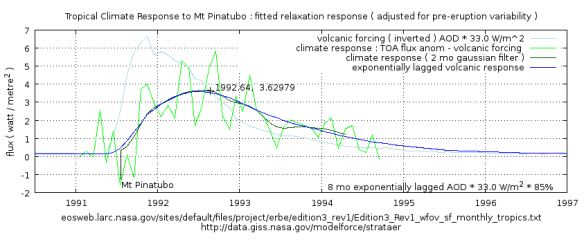
Figure 6 showing tropical feedback as relaxation response to volcanic aerosol forcing ( pre-eruption cycle removed) ( Click to enlarge )
The delayed climatic response to radiative change corresponds to the negative quadrant in figure 3b of Spencer and Braswell (2011) [5] excerpted below, where temperature lags radiative change. It shows the peak temperature response lagging around 12 months behind the radiative change. The timing of this peak is in close agreement with TOA response in figure 6 above, despite SB11 being derived from later CERES ( Clouds and the Earth’s Radiant Energy System ) satellite data from the post-2000 period with negligible volcanism.
This emphasises that the value for the correlation in the SB11 graph will be under-estimated, as pointed out by the authors:
Diagnosis of feedback cannot easily be made in such situations, because the radiative forcing decorrelates the co-variations between temperature and radiative flux.
The present analysis attempts to address that problem by analysing the fully developed response.
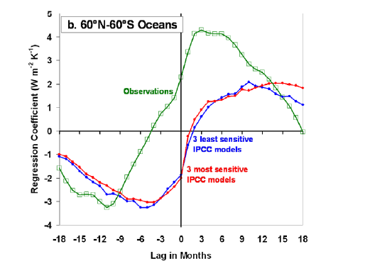
Figure 7. Lagged-correlation plot of post-2000 CERES data from Spencer & Braswell 2011. (Negative lag: radiation change leads temperature change.)
The equation of the relationship of the climate response : ( TOA net flux anomaly – volcanic forcing ) being proportional to an exponential regression of AOD, is re-arranged to enable an empirical estimation of the scaling factor by linear regression.
TOA -VF * AOD = -VF * k * exp_AOD eqn. 1
-TOA = VF * ( AOD – k * exp_AOD ) eqn. 2
VF is the volcanic scaling factor to convert ( positive ) AOD into a radiation flux anomaly in W/m2. The exp_AOD term is the exponential convolution of the AOD data, a function of the time-constant tau, whose value is also to be estimated from the data. This exp_AOD quantity is multiplied by a constant of proportionality, k. Since TOA net flux is conventionally given as positive downwards, it is negated in equation 2 to give a positive VF comparable to the values given by Lacis, Hansen, etc.
Average pre-eruption TOA flux was taken as the zero for TOA anomaly and, since the pre-eruption AOD was also very small, no constant term was included.
Since the relaxation response effectively filters out ( integrates ) much of high frequency variability giving a less noisy series, this was taken as the independent variable for regression. This choice acts to minimise regression dilution due to the presence of measurement error and non-linear variability in the independent variable.
Regression dilution is an important and pervasive problem that is often overlooked in published work in climatology, notably in attempts to derive an estimation of climate sensitivity from temperature and radiation measurements and from climate model output. Santer et al 2014, Trenberth et al 2010, Dessler 2011, Dessler 2010b, Spencer & Braswell 2011.
The convention of choosing temperature as the independent variable will lead to spuriously high sensitivity estimations. This was briefly discussed in the appendix of Forster & Gregory 2006 [11] , though ignored in the conclusions of the paper.
It has been suggested that a technique based on total least squares regression or bisector least squares regression gives a better fit, when errors in the data are uncharacterized (Isobe et al. 1990). For example, for 1985–96 both of these methods suggest YNET of around 3.5 +/- 2.0 W m-2 K-1 (a 0.7–2.4 K equilibrium surface temperature increase for 2 ϫ CO2), and this should be compared to our 1.0–3.6 K range quoted in the conclusions of the paper.
Regression results were thus examined for residual correlation.
Results
Taking the TOA flux, less the volcanic forcing, to represent the climatic reaction to the eruption, gives a response that peaks about twelve months after the eruption, when the stratospheric aerosol load is still at about 50% of its peak value. This implies a strong negative feedback is actively countering the volcanic disturbance.
This delay in the response, due to thermal inertia in the system, also produces an extended period during which the direct volcanic effects are falling and the climate reaction is thus greater than the forcing. This results in a recovery period, during which there is an excess of incoming radiation compared to the pre-eruption period which, to an as yet undetermined degree, recovers the energy deficit accumulated during the first year when the volcanic forcing was stronger than the developing feedback. This presumably also accounts for at least part of the post eruption maxima noted in the residuals of Santer et al 2014.
Thus if the lagged nature of the climate response is ignored and direct linear regression between climate variables and optical depth are conducted, the later extended period of warming may be spuriously attributed to some other factor. This represents a fundamental flaw in multivariate regression studies such as Foster & Rahmstorf 2013 [12] and Santer et al 2014 [8] , among others, that could lead to seriously erroneous conclusions about the relative contributions of the various regression variables.
For the case where the pre-eruption variation is assumed to continue to underlie the ensuing reaction to the volcanic forcing, the ratio of the relaxation response to the aerosol forcing is found to be 0.86 +/- 0.07%, with a time constant of 8 months. This corresponds to the value reported in Douglass & Knox 2005 [17] derived from AOD and lower troposphere temperature data. The scaling factor to convert AOD into a flux anomaly was found to be 33 W/m2 +/-11%. With these parameters, the centre line of the remaining 6 month variability ( shown by the gaussian filter ) fits very tightly to the relaxation model.
Figure 6 showing tropical feedback as relaxation response to volcanic aerosol forcing ( pre-eruption cycle removed) ( Click to enlarge )
If the downward trend in the pre-eruption data is ignored (ie its cause is assumed to stop at the instant of the eruption ) the result is very similar ( 0.85 +/-0.09 and 32.4 W/m2 +/- 9% ) but leads to a significantly longer time-constant of 16 months. In this case, the fitted response does not fit nearly as well, as can be seen by comparing figures 6 and 8. The response is over-damped: poorly matching the post-eruption change, indicating that the corresponding time-constant is too long.
 Figure 8 showing tropical climate relaxation response to volcanic aerosol forcing, fitted while ignoring pre-eruption variability. ( Click to enlarge )
The analysis with the pre-eruption cycle subtracted provides a generally flat residual ( figure 9 ), showing that it accounts well for the longer term response to the radiative disruption caused by the eruption.
It is also noted that the truncated peak, resulting from substitution of the mean of the annual cycle to fill the break in the ERBE satellite data, lies very close to the zero residual line. While there is no systematic deviation from zero it is clear that there is a residual seasonal effect and that the amplitude of this seasonal residual also seems to follow the fitted response.
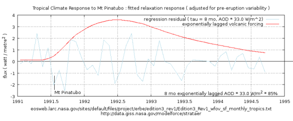 Figure 9 showing the residual of the fitted relaxation response from the satellite derived, top-of-troposphere disturbance. ( Click to enlarge )
Since the magnitude of the pre-eruption variability in TOA flux, while smaller, is of the same order as the volcanic forcing and its period similar to that of the duration of the atmospheric disturbance, the time-constant of the derived response is quite sensitive to whether this cycle is removed or not. However, it does not have much impact on the fitted estimation of the scaling factor ( VF ) required to convert AOD into a flux anomaly or the proportion of the exponentially lagged forcing that matches the TOA flux anomaly.
Assuming that whatever was causing this variability stopped at the moment of the eruption seems unreasonable but whether it was as cyclic as it appears to be, or how long that pattern would continue is speculative. However, approximating it as a simple oscillation seems to be more satisfactory than ignoring it.
In either case, there is a strong support here for values close to the original Lacis et al 1992 calculations of volcanic forcing that were derived from physics-based analysis of observational data, as opposed to later attempts to reconcile the output of general circulation models by re-adjusting physical parameters.
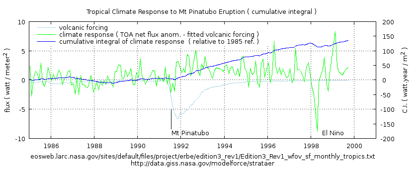
Beyond the initial climate reaction analysed so far, it is noted that the excess incoming flux does not fall to zero. To see this effect more clearly, the deviation of the flux from the chosen pre-eruption reference value is integrated over the full period of the data. The result is shown in figure 10.
 Figure 10 showing the cumulative integral of climate response to Mt Pinatubo eruption. ( Click to enlarge )
Pre-eruption variability produces a cumulative sum initially varying about zero. Two months after the eruption, when it is almost exactly zero, there is a sudden change as the climate reacts to the drop in energy entering the troposphere. From this point onwards there is an ever increasing amount of additional energy accumulating in the tropical lower climate system. With the exception of a small drop, apparently in reaction to the 1998 ‘super’ El Nino, this tendency continues to the end of the data.
While the simple relaxation model seems to adequately explain the initial four years following the Mt Pinatubo event, this does not explain it settling to a higher level. Thus there is evidence of a persisent warming effect resulting from this major stratospheric eruption.
Discussion
Concerning the more recent estimations of aerosol forcing, it should be noted that there is a strong commonality of authors in the papers cited here, so rather than being the work of conflicting groups, the more recent weightings reflect the result of a change of approach: from direct physical modelling of the aerosol forcing in the 1992 paper, to the later attempts to reconcile general circulation model (GCM) output by altering the input parameters.
From Hansen et al 2002 [4] ( Emphasis added. )
Abstract:
We illustrate the global response to these forcings for the SI2000 model with specified sea surface temperature and with a simple Q-flux ocean, thus helping to characterize the efficacy of each forcing. The model yields good agreement with observed global temperature change and heat storage in the ocean. This agreement does not yield an improved assessment of climate sensitivity or a confirmation of the net climate forcing because of possible compensations with opposite changes of these quantities. Nevertheless, the results imply that observed global temperature change during the past 50 years is primarily a response to radiative forcings.
Form section 2.2.2. Radiative forcing:
Even with the aerosol properties known, there is
uncertainty in their climate forcing. Using our SI2000
climate model to calculate the adjusted forcing for a
globally uniform stratospheric aerosol layer with optical
depth t = 0.1 at wavelength l = 0.55 mm yields a forcing of
2.1 W/m2 , and thus we infer that for small optical depths
Fa (W/m2) ~ 21 tau
…..
In our earlier 9-layer model stratospheric warming after El Chichon and Pinatubo was about half of observed values (Figure 5 of F-C), while the stratospheric warming in our current model exceeds observations, as shown below.
As the authors point out, it all depends heavily upon the assumptions made about size distribution of the aerosols used when interpreting the raw data. In fact the newer estimation is shown, in figure 5a of the paper, to be about twice the observed values following Pinatubo and El Chichon . It is unclear why this is any better than half observed values in their earlier work. Clearly the attributions are still highly uncertain and the declared uncertainty of +/-15% appears optimistic.
3.3. Model Sensitivity
The bottom line is that, although there has been some
narrowing of the range of climate sensitivities that emerge
from realistic models [Del Genio and Wolf, 2000], models
still can be made to yield a wide range of sensitivities by
altering model parameterizations.
If the volcanic aerosol forcing is underestimated, other model parameters will have to be adjusted to produce a higher sensitivity. It is likely that the massive overshoot in the model response of TLS is an indication of this situation. It would appear that a better estimation lies between these two extremes. Possibly around 25 W/m2.
The present study examines the largest and most rapid changes in radiative forcing in the period for which detailed satellite observations are available. The aim is to estimate the aerosol forcing and the timing of the tropical climate response. It is thus not encumbered by trying to optimise estimations of a range climate metrics over half a century by experimental adjustment of a multitude of “parameters”.
The result is in agreement with the earlier estimation of Lacis et al.
A clue to the continued excess over the pre-eruption conditions can be found in the temperature of the lower stratosphere, shown in figure 3. Here too, the initial disturbance seems to have stabilised by early 1995 but there is a definitive step change from pre-eruption conditions.
Noting the complementary nature of the effects of impurities in the stratosphere on TLS and the lower climate system, this drop in TLS may be expected to be accompanied by an increase in the amount of incoming radiation penetrating into the troposphere. This is in agreement with the cumulative integral shown in figure 10 and the southern hemisphere sea temperatures shown in figure 12.
NASA Earth Observatory report [13] that after Mt Pinatubo, there was a 5% to 8% drop in stratospheric ozone. Presumably a similar removal happened after El Chichon in 1982 which saw an almost identical reduction in TLS.
Whether this is, in fact, the cause or whether other radiation blocking aerosols were flushed out along with the volcanic emissions, the effect seems clear and consistent and quite specifically linked to the eruption event. This is witnessed in both the stratospheric and tropical tropospheric data. Neither effect is attributable to the steadily increasing GHG forcing which did not record a step change in September 1991.
This raises yet another possibility for false attribution in multivariate regression studies and in attempts to arbitrarily manipulate GCM input parameters to engineer a similarity with the recent surface temperature records.
With the fitted scaling factor showing the change in tropical TOA net flux matches 85% of the tropical AOD forcing, the remaining 15% must be dispersed elsewhere within the climate system. That means either storage in deeper waters and/or changes in the horizontal energy budget, ie. interaction with extra-tropical regions.
Since the model fits the data very closely, the residual 15% will have the same time dependency profile as the 85%, so these tropical/ex-tropical variations can also be seen as part of the climate response to the volcanic disturbance. ie. the excess in horizontal net flux, occurring beyond 12 months after the event, is also supporting restoration of the energy deficit in extra-tropical regions by exporting heat energy. Since the major ocean gyres bring cooler temperate waters into the eastern parts of tropics in both hemispheres and export warmer waters at their western extents, this is probably a major vector of this variation in heat transportation as are changes in atmospheric processes like Hadley convection.
Extra-tropical regions were previously found to be more sensitive to radiative imbalance that the tropics:
HadCRUT4 SH volcano stack cumulative sum of degree.days
Thus the remaining 15% may simply be the more stable tropical climate acting as a buffer and exerting a thermally stabilising influence on extra-tropical regions.
After the particulate matter and aerosols have dropped out there is also a long-term depletion of stratospheric ozone ( 5 to 8% less after Pinatubo ) [13]. Thompson & Solomon (2008) [14] examined how lower stratosphere temperature correlated with changes in ozone concentration and found that in addition to the initial warming caused by volcanic aerosols, TLS showed a notable ozone related cooling that persisted until 2003. They note that this is correlation study and do not imply causation.
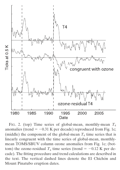
Figure 11. Part of fig.2 from Thompson & Solomon 2008 showing the relationship of ozone and TLS.
A more recent paper by Soloman [15] concluded roughly equal, low level aerosol forcing existed before Mt Pinatubo and again since 2000, similarly implying a small additional warming due to lower aerosols in the decade following the eruption.
Several independent data sets show that stratospheric aerosols have increased in abundance since 2000. Near-global satellite aerosol data imply a negative radiative forcing due to stratospheric aerosol changes over this period of about -0.1 watt per square meter, reducing the recent global warming that would otherwise have occurred. Observations from earlier periods are limited but suggest an additional negative radiative forcing of about -0.1 watt per square meter from 1960 to 1990.
The values for volcanic aerosol forcing derived here being in agreement with the physics-based assessments of Lacis et al. imply much stronger negative feedbacks must be in operation in the tropics than those resulting from the currently used model “parameterisations” and the much weaker AOD scaling factor.
These two results indicate that secondary effects of volcanism may have actually contributed to the late 20th century warming. This, along with the absence of any major eruptions since Mt Pinatubo, could go a long way to explaining the discrepancy between climate models and the relative stability of observational temperatures measurements since the turn of the century.
Once the nature of the signal has been recognised in the much less noisy stratospheric record, a similar variability can be found to exist in southern hemisphere sea surface temperatures. The slower rise in SST being accounted for by the much larger thermal inertia of the ocean mixed layer. Taking TLS as an indication of the end of the negative volcancic forcing and beginning of the additional warming forcing, the apparent relaxation to a new equilibrium takes 3 to 4 years. Regarding this approximately as the 95% settling of three times-constant intervals ( e-folding time ) would be consistent with a time constant of between 12 and 16 months for extra-tropical southern hemisphere oceans.
These figures are far shorter than values cited in Santer 2014 ranging from 30 to 40 months which are said to characterise the behaviour of high sensitivity models and correspond to typical IPCC values of climate sensitivity. It is equally noted from lag regression plots in S&B 2011 and Trenberth that climate models are far removed from observational data in terms of producing correct temporal relationships of radiative forcing and temperature.

Figure 12. Comparing SH sea surface temperatures to lower troposphere temperature.
Though the initial effects are dominated by the relaxation response to the aerosol forcing, both figures 9 and 12 show a additional climate reaction has a significant effect later. This appears to be linked to ozone concentration and/or a reduction in other atmospheric aerosols. While these changes are clearly triggered by the eruptions, they should not be considered part of the “feedback” in the sense of the relaxation response fitted here. These effects will act in the same sense as direct radiative feedback and shorten the time-constant by causing a faster recovery. However, the settling time of extra-tropical SST to the combined changes in forcing indicates a time constant ( and hence climate sensitivity ) well short of the figures produced by analysing climate model behaviour reported in Santer et al 2014 [8].
IPCC on Clouds and Aerosols:
IPCC AR5 WG1 Full Report Jan 2014 : Chapter 7 Clouds and Aerosols:
No robust mechanisms contribute negative feedback.
7.3.4.2
The responses of other cloud types, such as those associated with deep convection, are not well determined.
7.4.4.2
Satellite remote sensing suggests that aerosol-related invigoration of deep convective clouds may generate more extensive anvils that radiate at cooler temperatures, are optically thinner, and generate a positive contribution to ERFaci (Koren et al., 2010b). The global influence on ERFaci is
unclear.
Emphasis added.
WG1 are arguing from a position of self-declared ignorance on this critical aspect of how the climate system reacts to changes in radiative forcing. It is unclear how they can declare confidence levels of 95%, based on such an admittedly poor level of understanding of the key physical processes.
Conclusion
Analysis of satellite radiation measurements allows an assessment of the system response to changes in radiative forcing. This provides an estimation of the aerosol forcing that is in agreement with the range of physics-based calculations presented by Lacis et al in 1992 and is thus brings into question the much lower values currently used in GCM simulations.
The considerably higher values of aerosol forcing found here and in Lacis et al imply the presence of notably stronger negative feedbacks in tropical climate and hence imply a much lower range of sensitivity to radiative forcing than those currently used in the models.
The significant lag and ensuing post-eruption recovery period underlines the inadequacy of simple linear regression and multivariate regression in assessing the magnitude of various climate ‘forcings’ and their respective climate sensitivities. Use of such methods will suffer from regression dilution, omitted variable bias and can lead to seriously erroneous attributions.
Both the TLS cooling and the energy budget analysis presented here, imply a lasting warming effect on surface temperatures triggered by the Mt Pinatubo event. Unless these secondary effects are recognised, their mechanisms understood and correctly modelled, there is a strong likelihood of this warming being spuriously attributed to some other cause such as AGW.
When attempting to tune model parameters to reproduce the late 20th century climate record, an incorrectly small scaling of volcanic forcing, leading to a spuriously high sensitivity, will need to be counter-balanced by some other variable. This is commonly a spuriously high greenhouse effect, amplified by presumed positive feedbacks from other climate variables, less well constrained by observation ( such as water vapour and cloud ). In the presence of the substantial internal variability, this can be made to roughly match the data while both forcings are present ( pre-2000 ). However, in the absence of significant volcanism there will be a steadily increasing divergence. The erroneous attribution problem, along with the absence of any major eruptions since Mt Pinatubo, could explain much of the discrepancy between climate models and the relative stability of observational temperature measurements since the turn of the century.
References:
[1] Self et al 1995
“The Atmospheric Impact of the 1991 Mount Pinatubo Eruption”
http://pubs.usgs.gov/pinatubo/self/
[2] Lacis et al 1992 : “Climate Forcing by Stratospheric Aerosols
Click to access 1992_Lacis_etal_1.pdf
[3] Hansen et al 1997 “Forcing and Chaos in interannual to decadal climate change”
Click to access Hansen_etal_1997b.pdf
[4] Hansen et al 2002 : “Climate forcings in Goddard Institute for Space Studies SI2000 simulations”
Click to access hansen_etal_2002.pdf
[5] Spencer & Braswell 2011: “On the Misdiagnosis of Surface Temperature Feedbacks from Variations in Earth’s Radiant Energy Balance”
http://www.mdpi.com/2072-4292/3/8/1603/pdf
[6] Lindzen & Choi 2011: “On the Observational Determination of Climate Sensitivity and Its Implications”
Click to access 236-Lindzen-Choi-2011.pdf
[7] Trenberth et al 2010: “Relationships between tropical sea surface temperature and top‐of‐atmosphere radiation”
http://www.mdpi.com/2072-4292/3/9/2051/pdf
[8] Santer et al 2014: “Volcanic contribution to decadal changes in tropospheric temperature”
http://www.nature.com/ngeo/journal/v7/n3/full/ngeo2098.html
[8b] Supplementary Information:
Click to access ngeo2098-s1.pdf
[9] Dessler 2010 b “A Determination of the Cloud Feedback from Climate Variations over the Past Decade”
Click to access dessler10b.pdf
[10] Dessler 2011 “Cloud variations and the Earth’s energy budget”
Click to access Dessler2011.pdf
[11]Forster & Gregory 2006
“The Climate Sensitivity and Its Components Diagnosed from Earth Radiation Budget Data”
Click to access Forster_sensitivity.pdf
[12] Foster and Rahmstorf 2011: “Global temperature evolution 1979-2010”
http://stacks.iop.org/ERL/6/044022
[13] NASA Earth Observatory
http://earthobservatory.nasa.gov/Features/Volcano/
[14] Thompson & Soloman 2008: “Understanding Recent Stratospheric Climate Change”
http://journals.ametsoc.org/doi/abs/10.1175/2008JCLI2482.1
[15] Susan Soloman 2011: “The Persistently Variable “Background” Stratospheric Aerosol Layer and Global Climate Change”
http://www.sciencemag.org/content/333/6044/866
[16] Trenberth 2002: “Changes in Tropical Clouds and Radiation”
Click to access 2095.full.pdf
[17] Douglass & Knox 2005: “Climate forcing by the volcanic eruption of Mount Pinatubo”
Click to access 2004GL022119_Pinatubo.pdf
[18] Douglass & Knox 2005b: “Reply to comment by A. Robock on ‘‘Climate forcing by the volcanic eruption of Mount Pinatubo’’”
Click to access reply_Robock_2005GL023829.pdf
Data sources:
[DS1] AOD data: NASA GISS
http://data.giss.nasa.gov/modelforce/strataer
Derived from SAGE (Stratospheric Aerosol and Gas Experiment) instrument.
“The estimated uncertainty of the optical depth in our multiple wavelength retrievals [Lacis et al., 2000] using SAGE observations is typically several percent. “[4]
[DS2] ERBE TOA data: Earth Radiation Budget Experiment
http://eosweb.larc.nasa.gov/sites/default/files/project/erbe/edition3_rev1/Edition3_Rev1_wfov_sf_monthly_tropics.txt
data description:
Click to access erbe_s10n_wfov_nf_sf_erbs_edition3.pdf
[*] Explanatory notes:
Negative feedback is an engineering term that refers to a reaction that opposes its cause. It is not a value judgement about whether it is good or bad. In fact, negative feedbacks are essential in keeping a system stable. Positive feedbacks lead to instability and are thus generally “bad”.
Convolution is a mathematical process that is used, amongst other things, to implement digital filters. A relaxation response can be implemented by convolution with an exponential function. This can be regarded as an asymmetric filter with a non-linear phase response. It produces a delay relative to the input and alters it’s shape.
Regression dilution refers to the reduction in the slope estimations produced by least squares regression when there is significant error or noise in the x-variable. Under negligible x-errors OLS regression can be shown to produce the best unbiased linear estimation of the slope. However, this essential condition is often over-looked or ignored, leading to erroneously low estimations of the relationship between two quantities. This is explained in more detail here:
On inappropriate use of least squares regression
Supplementary Information
Detailed method description.
The break of four months in the ERBE data at the end of 1993 was filled with the anomaly mean for the period to provide a continuous series. This truncates what would have probably been a small peak in the data, marginally lowering the local average, but since this was not the primary period of interest this short defect was considered acceptable.
The regression was performed for a range of time-constants from 1 to 24 months. The period for the regression was from just before the eruption, up to 1994.7, when AOD had subsided and the magnitude of the annual cycle was found to change, indicating the end of the initial climatic response ( as determined from the adaptive anomaly shown in figure 2 ).
Once the scaling factor was obtained by linear regression for each value of tau, the values were checked for regression dilution by examining the correlation of the residual of the fit with the AOD regressor while varying the value of VF in the vicinity of the fitted value. This was found to give a regular curve with a minimum correlation that was very close to the fitted value. It was concluded that the least squares regression results were an accurate estimation of the presumed linear relationship.
The low values of time-constant resulted in very high values of VF ( eg. 154 for tau=1 month ) that were physically unrealistic and way out side the range of credible values. This effectively swamps the TOA anomaly term and is not meaningful.
tau = 6 months gave VF = 54 and this was taken as the lower limit for the range time constant to be considered.
The two free parameters of the regression calculations will ensure an approximate fit of the two curves for each value of the time constant. The latter could then be varied to find the response that best fitted the initial rise after the eruption, the peak and the fall-off during 1993-1995.
This presented a problem since, even with adaptive anomaly approach, there remains a significant, roughly cyclic, six month sub-annual variability that approaches in magnitude the climate response of interest. This may be at least in part a result aliasing of the diurnal signal to a period close to six months in the monthly ERBE data as pointed out by Trenberth [16]. The relative magnitude of the two also varies depending on the time-constant used, making a simple correlation test unhelpful in determining the best correlation with respect to the inter-annual variability. For this reason it could not be included as a regression variable.
Also the initial perturbation and the response, rise very quickly from zero to maximum in about two months. This means that low-pass filtering to remove the 6 month signal will also attenuate the initial part of the effect under investigation. For this reason a light gaussian filter ( sigma = 2 months ) was used. This has 50% attenuation at 2.3 months. comparable to a 4 month running mean filter ( without the destructive distortions of the latter). This allowed a direct comparison of the rise, duration of the peak and rate of fall-off in the tail that is determined by the value of the time-constant parameter, and thus the value producing the best match to the climate response.
Due to the relatively course granularity of monthly data that limits the choice of the time-constant values, it was possible to determine a single value that produced the best match between the two variables.
The whole process was repeated with and without subtraction of the oscillatory, pre-eruption variability to determine the effects of this adjustment.
The uncertainty values given are those of the fitting process and reflect the variability of the data. They do not account for the experimental uncertainty in interpreting the satellite data.
Beyond the single slab model.
A more complex model which includes a heat diffusion term to a large deep ocean sink can be seen to reduce to the same analytical form with a slightly modified forcing and an increased “effective” feedback. Both these adjustments would be small and do not change the mathematical form of the equation and hence the validity of the current method.
A typical representation of the linear model used by many authors in published works [17] is of the form:
C *d/dt(Ts) = F – λTs
where Ts is surface temp anomaly ; F is radiative flux anomaly and C is the heat capacity of the mixed ocean layer. λ is a constant which is the reciprocal of climate sensitivity.
Eddy diffusion anomaly to the deep ocean heat sink at a constant temperature Td can be added using a diffusion constant κ With the relatively small changes in surface temperature over the period compared to the surface – thermocline temperature difference in the tropics, the square law of the diffusion equation can be approximated as linear. To within this approximation, a two slab diffusion model has the same form as signle slab model.
A simple rearrangement shows that this is equivalent to original model but with a slightly modified flux and an slightly increased feedback parameter.
C *d/dt(Ts) + κ*(Ts-Td) = F – λTs
C *d/dt(Ts) = F – λTs- κ*(Ts-Td)
C *d/dt(Ts) = F+ κ*(Td) – Ts(λ+κ)
This does not have a notable effect on the scaling of the volcanic forcing herein derived, nor the presence of the anomalous, post-eruption warming effect, which is seen to continue beyond the period of the AOD disruption and the topical climate resposne.