Derivative-of-Gaussian filter

The following awk script will apply a gaussian filter to the rate of change ( derivative ) of the data.  This is simpler than doing two separate operations and provides a more accurate numerical estimation of the derivative than using two point “first difference”.

Since we know the analytical form of the derivative of the gaussian function, the derivative can be applied before making a quantised approximation for numerical processing of quantised data.

Analytically, since both the convolution and the derivative are linear operations they can be done in either order and produce identical results. This allows taking the derivative of the gaussian then doing a single convolution without loss of generality.

There is still the inaccuracy of approximating the infinite gaussian function by a finite, quantised kernel but there is no loss of accuracy from also approximating the derivative. Thus the result is mathematically more accurate than using the first difference and then a gaussian filter.

The usual 3-sigma window for a gaussian filter is slightly extended to maintain similar accuracy in the D-o-G filter.

Since the derivate has high-pass properties ( attenuation inversely proportional to frequency ) and the gaussian is a low-pass filter the combined filter is a band pass filter. One common use if for edge detection, for example in medical imagery. Equally if the derivative of the data is being studied and some low-pass filtering is required it provides a one-step solution that does not rely on a digitised approximation of the derivative.

An example of edge detection is shown in determining long-term variations in the date of Arctic sea-ice minima:

The Death Spiral is Dead


Select and copy the text in the following block to get a copy of the script.


#!/bin/awk -f
# 3-sigma derviative of gaussian filter
# sigma, if not given, is 2 data points wide
# usage : ./dgauss.awk filename <sigma=2> <scale_factor=1>
# optional scale_factor simply scales the output
# sigma can be compared to the period of the -3dB point of the filter
# result is centred, ie not phase shifted. resulting dataset shorter by 3*sigma ( half window ) each end
# nov 2012 OFMT="%10.8f"


### ensure data is continuous and equally spaced ### !!


# FWHM (-3dB) = 2*sigma*sqrt(2*ln2)
# half height freq = sigma * 1.1774
# 3 sigma gives 99.7% accuracy for gauss, extend to 4-sigma for deriv-gauss

function abs(x){return (((x < 0.0) ? -x : x) + 0.0)}

BEGIN { OFMT="%10.8f"
# ARGV[1]=filename; argv[0] is script name, hence ARGC>=1

 datacol=2 # fixed

 if (ARGV[1]=="") { print " # usage : ./dgauss.awk filename <sigma=2> <scale_factor=1>" ; exit 1}

 pi= 3.14159265359811668006

 if ( ARGC >3 ) {scaleby=ARGV[3];ARGV[3]=""} else {scaleby=1};
 if ( ARGC >2 ) {sigma=ARGV[2];ARGV[2]=""} else {sigma=2};

 print "# filtering "ARGV[1]" with gaussian-derivative of sigma= ",sigma
 root2pi_sigma=sqrt(2*pi)*sigma;
 two_sig_sqr=2.0*sigma*sigma;

# extend 3 sigma window to 3.5 for derivate-gauss to maintain accuracy.
 gw=(4*sigma)-1;

# calculate normalised gaussian coeffs
# for (tot_wt=j=0;j<=gw;j++) {tot_wt+=gwt[-j]=gwt[j]=exp(-j*j/two_sig_sqr)/ root2pi_sigma};
# tot_wt=0

### NB d/dt(gauss) is asymmetric, so must be time reversed to correctly do convolution.
 for (tot_wt=j=0;j<=gw;j++) {tot_wt+=gwt[j]= j/sigma/sigma*exp(-j*j/two_sig_sqr) / root2pi_sigma };
 tot_wt=2*tot_wt-gwt[0]; # to scale each lobe to |0.5| ; gwt[0]=0
 tot_wt/=scaleby;
 for (j=0;j<=gw;j++) {
# gwt[j]/=tot_wt; # gaussian is already normalised, don't rescale derivate !
 gwt[-j]=-gwt[j]
 };

# strip off last .xxx part of file name
# FIXME : improve this (doesn't work with paths like ../filename)

 if (ARGV[1]=="-") {
 out_file="-";
 }
 else {
 split(ARGV[1],fn,".");
 basename=fn[1]
 out_file=basename"-gauss-deriv"sigma".dat";
 print "# ",out_file >out_file;
 }

 ln=-1;
}

( ($0 !~ /^#/) && ($0 !~ /^[" ",\t]*$/) ) {
 xdata[++ln]=$1;
 ydata[ln]=$datacol;

 if (ln>2*gw)
 {

# cf diff.awk
# print (xdata[ln]+xdata[ln-step])/2. ,ydiff/xdiff
# print (xdata[ln]+xdata[ln-step])/2. ,ydiff/xdiff >> out_file;

 xdiff=(xdata[ln]-xdata[ln-1]);
# ydiff=(ydata[ln]-ydata[ln-step]);

 dgauss=0
 for (j=-2*gw;j<=0;j++) {dgauss+=ydata[ln+j]*gwt[j+gw]}
 if (out_file=="-")
   print xdata[ln-gw],dgauss/xdiff , ydata[ln-gw] 
 else {
   print NR,xdata[ln-gw],dgauss/xdiff ,ydata[ln-gw]
   print xdata[ln-gw],dgauss/xdiff , ydata[ln-gw] >> out_file;
  }
 }
else
 {
# print $1,$2;

 }
}


END {
 if (ARGV[1]=="") { exit 1}
 print "# gausssian-derivative window width = "gw+gw+1",done"
 print "# output file = "out_file
 # sum=0; for (j=-gw;j<=gw;j++) {sum+= abs(gwt[j]);}
 # print "# abs sum of coeffs = ",sum;

}

Triple running mean filter

The following script will call a simple running mean three times with appropriate window size to do effect triple running mean, as described in the article (as amended for the asymmetric kernel to minimise negative leakage):

Data corruption by running mean “smoothers”

It requires the runmean.awk script found here:

simple running-mean script ( as base for triple RM )

Select code with mouse to copy elsewhere.

#!/bin/bash

# call runmean.awk three times to compose triple running mean
# usage: ./r3m.sh file window_len   ; default window is 12 data point

if [ "x$1" == "x"  ]; then echo "$0 : err no file name,   usage: $0 filename "
 exit 1;
else fn=$1
fi

if [ "x$2" == "x"  ]; then win=12; else win=$2; fi

#win2=`awk "BEGIN{print $win/ 1.3371}"`
#win3=`awk "BEGIN{print $win/ 1.3371/ 1.3371}"`

# asymmetric stages with following window ratios minimise neg. lobe in freq. response
k=1.15; k2=1.58

win2=`awk "BEGIN{print $win/ "$k"}"`
win3=`awk "BEGIN{print $win/ "$k2" }"`

outfile=`echo $fn | awk '{ print substr($1,1,length($1)-4) }'`
outfile+="-3rm"$win".dat"

echo  "# triple running mean :  $win  $win2  $win3 " > $outfile

# echo $fn; echo $win; echo $win2; echo $win3

cat $fn | ./runmean.awk - $win |  ./runmean.awk - $win2 |  ./runmean.awk - $win3 >> $outfile

#echo "# cat $fn | ./runmean.awk - $win |  ./runmean.awk - $win2 |  ./runmean.awk - $win3 >> $outfile"

echo "# triple running mean :  $win  $win2  $win3 "
echo "# outfile = "$outfile;

Gaussian low-pass filter


Click to enlarge graph.

The graph is scaled to unit frequency (eg 1 Hz or one cycle per year …).

It illustrates how a 159 day gaussian will filter daily data. For monthly data 12*159/365=5.23 , so the nearest would be sigma=5mo . However since that is slightly short of the intended value and gaussian leaks a little, since it is never fully zero, six months would be better to suppress a 12mo cycle.

Code ( use copy / paste within code block ).

There must be NO space before the first line. ie “#!” are the first characters in the file.

#!/bin/awk -f

# pass input through 3 sigma gaussian filter where sigma, if not given, is 2 data points wide
# usage : ./gauss.awk filename <sigma=2> <scale_factor=1>
# optional scale_factor simply scales the output
# sigma can be compared to the period of the -3dB point of the filter
# result is centred, ie not shift. dataset shortened by half window each end

# operates on files with two columns of numeric data, or a single column of data
#  eg date as integer year or floating point decimal
# single column takes line number position to be evenly spaced ordinate variable.
# ensure that data is equally spaced and continuous !!
# nov 2012  OFMT="%10.8f"

# 159d gauss similar to  365d r3m

# FWHM (-3dB) = 2*sigma*sqrt(2*ln2)
# half height freq = sigma * 1.1774
# 3 sigma gives 99.7% accuracy

BEGIN { OFMT="%10.8f"
# ARGV[1]=filename; argv[0] is script name, hence ARGC>=1

  if (ARGV[1]=="") { print " # usage : ./gauss.awk filename <sigma=2> <scale_factor=1>" ; exit 1}

  pi= 3.14159265359811668006

  if  ( ARGC >3 ) {scaleby=ARGV[3];ARGV[3]=""} else {scaleby=1};
  if  ( ARGC >2 ) {sigma=ARGV[2];ARGV[2]=""} else {sigma=2};

  print "# filtering "ARGV[1]" with gaussian of sigma= ",sigma
  root2pi_sigma=sqrt(2*pi)*sigma;
  two_sig_sqr=2.0*sigma*sigma;

  gw=3*sigma-1;  # gauss is approx zero at 3 sigma, use 3 sig window

# calculate normalised gaussian coeffs
  for (tot_wt=j=0;j<=gw;j++) {tot_wt+=gwt[-j]=gwt[j]=exp(-j*j/two_sig_sqr)/ root2pi_sigma};
  tot_wt=2*tot_wt-gwt[0];
  tot_wt/=scaleby;
  for (j=-gw;j<=gw;j++) {gwt[j]/=tot_wt};

# strip off last .xxx part of file name
# improve this  (doesn't work with paths like ../filename)

  if (ARGV[1]=="-") {
    out_file="-";
  }
   else {
    split(ARGV[1],fn,".");
    basename=fn[1]
    out_file=basename"-gauss"sigma".dat";
    print "# ",out_file >out_file;
  }

  ln=-1;
}

( ($0 !~ /^#/) && ($0 !~ /^[" ",\t]*$/)  ) {
  xdata[++ln]=$1;
  ydata[ln]=$2;  

  if (ln>2*gw)
  {
    gauss=0
    for (j=-2*gw;j<=0;j++) {gauss+=ydata[ln+j]*gwt[j+gw]}
    if (out_file=="-")
      print xdata[ln-gw],gauss
    else {
      print NR,xdata[ln-gw],gauss
      print xdata[ln-gw],gauss >> out_file;
    }
  }
}

END {
  if (ARGV[1]=="") { exit 1}
  print "# gausssian window width = "gw+gw+1",done"
  print "# output file = "out_file

# for (i=0;i<=gw;i++){print gwt[i]}
}

Lanczos high-pass filter


The graph shows the frequency response of a 3-lobe Lanczos high-pass filter with central frequencies of 461 and 269 days, respectively.

These are chosen such that a periodicity of 1 year is either fully included or fully excluded in the filter’s pass-band. ie the 269 day filter will pass only frequencies shorter than 365 days and fully block annual cycles. 461 day filter will ensure that everything including the annual signal is unattenuated and excludes anything longer than about 1.6 years.

The equivalent low-pass filter is detailed here:

Lanczos low-pass filter

frequency axis is in units of “per year” not “year” as labelled.

Code: ( select text in code block and use copy/paste to get the code )

#!/bin/awk -f

#  usage: ./lanczos_HP.awk filename [-3dB_period=17] [lobes=3]"

# purpose: apply a high-pass filter by convolution of 2nd column of file with lanczos windowed sinc function
# column 1 data should be evenly spaced without gaps.
# optional second parameter is period of 3dB attenuation, as a period expressed  in data intervals
#    default = 17 ; eg. 17 monthly periods : half power at 17mo, close to 100% pass at 12 mo.
#                   to exclude 12mo, use 9 . This will pass 6mo and higher freq unattenuated.
#                   for daily data use 461 and 269 days , respectively.
# optional third parameter is the number of lobes in impulse response. More gives sharper transition but can produce overshoot ( ringing $
# comments at end of output give pass-band and stop band info, this is not sent to output file.
#    default=3; 4 is OK. ### >=5 may produce significant ringing artefacts around sharp, high amplitude changes###


function sinc(x) {
  if (x==0) return 1; else return (sin(x)/x);
}

BEGIN{  OFMT = "%8.6f"

  twopi=6.28318530717959

  if ( ARGC >3 ) {lobes=ARGV[3];ARGV[3]=""} else {lobes=3};
  if ( ARGC >2 ) {period=ARGV[2];ARGV[2]=""} else {period=17};
  if ( ARGC <2) { print "### usage: ./lanczos_HP.awk filename [-3dB_period=17] [lobes=3]"; err=1; exit 1; }
  else {len=ARGV[2]; ARGC=2;}

  pi= 3.14159265359811668006 ;
  halfk=int(period/2*lobes);
  kwid= 2*halfk;         # kernel = -halfk....+halfk = kwid+1 pts ie odd number
  w_taper=twopi/kwid;    # first lanczos lobe -pi to +pi to fill window
  w=twopi/period;        # sinc passes zero pi, 2*pi, 3*pi ....

# calculate normalised kernel coeffs
  for (tot_wt=j=0;j<=halfk;j++) {tot_wt+=gwt[-j]=gwt[j]=sinc(j*w)*sinc(j*w_taper)};
  tot_wt=2*tot_wt-gwt[0];

# for HP filter, invert LP and add unit impulse:
  for (j=-halfk;j<=halfk;j++) {gwt[j]/=-tot_wt};
  gwt[0]+=1;

# strip off last .xxx part of file name
# improve this  (doesn't work with paths like ../filename)


  if (ARGV[1]=="-") {
    out_file="-";
  }
  else {
    split(ARGV[1],fn,".");
    for (i=1;i<length(fn);i++){   # if multiple dots in name, build back up except last part
      if(i==1)basename=fn[i]
      else basename=basename"."fn[i];
    }
    out_file=basename"-lanc"lobes"HP_"period".dat";
    print "# ",out_file >out_file;
    print "# ",out_file
  }

  ln=-1;  # init linenumber counter
}

($0 !~ /^#/)&&($0 != "") {    # strip out comments, headers and blank lines
  xdata[++ln]=$1;
  ydata[ln]=$2;

  if (ln>2*halfk)
  {
    sum=0
    for (j=-2*halfk;j<=0;j++) {sum+=ydata[ln+j]*gwt[j+halfk]}
    if (out_file=="-")
      print xdata[ln-halfk],sum
    else {
      print NR,xdata[ln-halfk],sum
      print xdata[ln-halfk],sum >> out_file;
    }
  } #endif ln

}


END {
    if (err) exit err;
    if (FNR<=kwid) {print " ### insufficient data to fill "kwid+1" point filter buffer"; exit 1}
    print "# "lobes"-lobe lanczos kernel width = "2*halfk+1",done"
    if (lobes==5) printf ("# "lobes"-lobe lanczos HP on %s: zero-pass > %.3f; 99% pass < %.3f \n",ARGV[1],period/.752,period/1.258)
    if (lobes==4) printf ("# "lobes"-lobe lanczos HP on %s: zero-pass > %.3f; 99% pass < %.3f \n",ARGV[1],period/.698,period/1.325)
    if (lobes==3) printf ("# "lobes"-lobe lanczos HP on %s: zero-pass > %.3f; 99% pass < %.3f \n",ARGV[1],period/.588,period/1.436)

    print "# output file = "out_file
# uncomment following to dump kernel (impluse response):
# sum=0; for (j=-halfk;j<=halfk;j++) {sum+= gwt[j]; printf ("%.4f\n", gwt[j])}
# print "# abs sum of coeffs = ",sum;

}


Lanczos low-pass filter


Click to enlarge graph.

frequency axis is in units of “per year” not “year” as labelled.

Equivalent high-pass filter:

Lanczos high-pass filter

Discussion: https://climategrog.wordpress.com/?attachment_id=659

Source Code: ( to get code, use browser copy / paste function within code block below).

#!/bin/awk -f

#  usage: ./lanczos_LP.awk filename [50%_attn_period=18] [lobes=3]"

# purpose: convolve 2nd column of file with lanczos windowed sinc function
# this provides low-pass filter with a fast transition from pass-band to stop-band , with minimal ripple in both.
# column 1 data should be evenly spaced without gaps.
# optional second parameter is period of 50% attenuation, as a period expressed in data intervals
# optional third parameter is the number of lobes in impulse response.
# zero pass req period * 1.436 eg 17.23mo or 525 days
#    default=18 ; eg. 18 monthly periods : 50% attenuation at 15mo, close to zero pass at 12 mo. for 3 lobe.
#    lobes=3 ; use 525 for daily ; lobes=5 ; use 461 for 365 data
# console output comments give pass-band and stop band info. this is not sent to output file.

#    More lobes gives sharper transition band but more overshoot distortion / ringing.
#    default=3; 3 and 4 are good. ### >=5 may produce significant ringing artefacts ###


function sinc(x) {
  if (x==0) return 1; else return (sin(x)/x);
}

BEGIN{  OFMT = "%8.6f"


  if ( ARGC >3 ) {lobes=ARGV[3];ARGV[3]=""} else {lobes=3};
  if ( ARGC >2 ) {period=ARGV[2];ARGV[2]=""} else {period=18};
  if ( ARGC <2) { print "### usage: ./lanczos_LP.awk filename [50%_attn_period=18] [lobes=3]"; err=1; exit 1; }
  else {len=ARGV[2]; ARGC=2;}

  pi= 3.14159265359811668006 ;
  twopi=2*pi;
  halfk=int(period/2*lobes);
  kwid= 2*halfk;         # kernel = -halfk....+halfk = kwid+1 pts ie odd number
  w_taper=twopi/kwid;    # first lanczos lobe -pi to +pi to fill window
  w=twopi/period;        # sinc passes zero pi, 2*pi, 3*pi ....

# calculate normalised kernel coeffs
  for (tot_wt=j=0;j<=halfk;j++) {tot_wt+=gwt[-j]=gwt[j]=sinc(j*w)*sinc(j*w_taper)};
  tot_wt=2*tot_wt-gwt[0];
  for (j=-halfk;j<=halfk;j++) {gwt[j]/=tot_wt};

# strip off last .xxx part of file name
# improve this  (doesn't work with paths like ../filename)

  if (ARGV[1]=="-") {
    out_file="-";
  }
  else {
    split(ARGV[1],fn,".");
    for (i=1;i<length(fn);i++){   # if multiple dots in name, build back up except last part
      if(i==1)basename=fn[i]
      else basename=basename"."fn[i];
    }
    out_file=basename"-lanc"lobes"LP_"period".dat";
    print "# ",out_file >out_file;
    print "# ",out_file
  }

  ln=-1;  # init linenumber counter
}

($0 !~ /^#/)&&($0 != "") {    # strip out comments, headers and blank lines
  xdata[++ln]=$1;
  ydata[ln]=$2;

  if (ln>2*halfk)
  {
    sum=0
    for (j=-2*halfk;j<=0;j++) {sum+=ydata[ln+j]*gwt[j+halfk]}
    if (out_file=="-")
      print xdata[ln-halfk],sum
    else {
      print NR,xdata[ln-halfk],sum
      print xdata[ln-halfk],sum >> out_file;
    }
  } #endif ln

}


END {
    if (err) exit err;
    if (FNR<=kwid) {print " ### insufficient data to fill "kwid+1" point filter buffer"; exit 1}
    print "# "lobes"-lobe lanczos kernel width = "2*halfk+1",done"
    if (lobes==5) printf ("# "lobes"-lobe lanczos LP on %s: zero-pass at %.3f; 99% pass > %.3f \n",ARGV[1],period/1.258,period/.752)
    if (lobes==4) printf ("# "lobes"-lobe lanczos LP on %s: zero-pass at %.3f; 99% pass > %.3f \n",ARGV[1],period/1.325,period/.698)
    if (lobes==3) printf ("# "lobes"-lobe lanczos LP on %s: zero-pass at %.3f; 99% pass > %.3f \n",ARGV[1],period/1.436,period/.588)

    print "# output file = "out_file
# uncomment following to dump kernel (impluse response):
# sum=0; for (j=-halfk;j<=halfk;j++) {sum+= gwt[j]; printf ("%.4f\n", gwt[j])}
# print "# abs sum of coeffs = ",sum;

}

simple running-mean script ( as base for triple RM )

The following script will calculate a simple running mean. On its own this is a very poor filter, see accompanying article :

Data corruption by running mean “smoothers”

This script is intended for use by the triple-running-mean script available here:

triple running-mean filter

Select code with mouse to copy elsewhere.

#!/bin/awk -f

# calculate running mean of width 'window'
# line number taken as x if file if file is a single column of data
# [usage] ./runmean.awk filename <window>
# default window=12
# strips empty and comment lines

# operates on files with two columns of numeric data
#  eg date as integer year or floating point decimal
# check whether data is continuous and evenly spaced !!


BEGIN{  OFMT = "%10.8f"
# ARGV[1]=fn; argv[0] is script name, hence ARGC>=1

  if (ARGV[1]=="") { print " ### error, no input file given." ; err=1; exit 1}

  ln=0;
  if  ( ARGC >2 ) {window=ARGV[2];ARGV[2]=""} else {window=12};
  if (int(window)!=window) {window=int(window+0.5); window_adj=1; }

  print "# filtering "ARGV[1]" with running mean  window = ",window

  if (ARGV[1]=="-") {
    out_file="-";
  }
   else {
    split(ARGV[1],fn,".");
    basename=fn[1]
    out_file=basename"-rmean"window".dat";

    print "# ",out_file >out_file;
  }
}  # end BEGIN


{ # body
if ( ($0 !~ /^#/) && ($0 !~ /^[" ",\t]*$/)  )  {  # strip empty and comment lines

  if ($2==""){  # for single column data files
    xdata[++ln]=NR;
    ydata[ln]=$1;
  }else{
    xdata[++ln]=$1;
    ydata[ln]=$2;
  }

  sum+=ydata[ln];

  if (ln>=window)
  {
    mid_x=(xdata[ln]+xdata[ln-(window-1)])/2;  # -1 to centre correctly
    ymean=(sum)/window;
    sum-= ydata[ln-window+1];  # remove oldest
    if (out_file=="-")
      print mid_x,ymean;
    else {
      print NR,mid_x,ymean
      print mid_x,ymean >> out_file;
    }
  } # endif
 } # non empty
} # end body

END {
  if (err==1) { exit 1}
  if (window_adj==1) print "# warning : window rounded to nearest integer, window  = ",window
  print "# running mean window = "window",done"
  print "# output file = "out_file
}

triple running-mean filter

The following script will call a simple running mean three times with appropriate window size to do effect triple running mean, as described in the article (as amended for the asymmetric kernel to minimise negative leakage):

Data corruption by running mean “smoothers”

It requires the runmean.awk script found here:

simple running-mean script ( as base for triple RM )

Select code with mouse to copy elsewhere.

#!/bin/bash

# call runmean.awk three times to compose triple running mean
# usage: ./r3m.sh file window_len   ; default window is 12 data point

if [ "x$1" == "x"  ]; then echo "$0 : err no file name,   usage: $0 filename "
 exit 1;
else fn=$1
fi

if [ "x$2" == "x"  ]; then win=12; else win=$2; fi

#win2=`awk "BEGIN{print $win/ 1.3371}"`
#win3=`awk "BEGIN{print $win/ 1.3371/ 1.3371}"`


# asymmetric stages with following window ratios:
k=1.15; k2=1.58

win2=`awk "BEGIN{print $win/ "$k"}"`
win3=`awk "BEGIN{print $win/ "$k2" }"`

outfile=`echo $fn | awk '{ print substr($1,1,length($1)-4) }'`
outfile+="-3rm"$win".dat"

echo  "# triple running mean :  $win  $win2  $win3 " > $outfile

# echo $fn; echo $win; echo $win2; echo $win3

cat $fn | ./runmean.awk - $win |  ./runmean.awk - $win2 |  ./runmean.awk - $win3 >> $outfile

#echo "# cat $fn | ./runmean.awk - $win |  ./runmean.awk - $win2 |  ./runmean.awk - $win3 >> $outfile"

echo "# triple running mean :  $win  $win2  $win3 "
echo "# outfile = "$outfile;

Data corruption by running mean “smoothers”

[See update at end of article]

Running means are often used as a simple low pass filter (usually without understanding its defects). Often it is referred to as a “smoother”. In fact it does not even “smooth” too well either since it lets through enough high frequencies to give a spiky result.

Running means are fast and easy to implement. Since most people have some understanding of what an average does, the idea of a running average seems easily understood. Sadly it’s not that simple and running averages often cause serious corruption of the data.

So it smooths the data to an extent, but what else does it do?

The problem with an evenly weighted average is that the data is effectively masked by a rectangular window. The frequency response of such a rectangular window is the sinc function [1] and thus the effect on the frequency content of the data is to apply the sinc function as a frequency filter. The sinc function oscillates and has negative lobes that actually invert part of the signal it was intended to remove. This can introduce all sorts of undesirable artefacts into the data.

An example of one of the problems can be seen here:
running_mean_WTF
http://www.woodfortrees.org/plot/rss/from:1980/plot/rss/from:1980/mean:60/plot/rss/from:1980/mean:30/mean:22/mean:17
Figure 1 Comparing effects of different filters on a climate data time series ( 60 month running mean vs 30m triple running mean [blue] ).

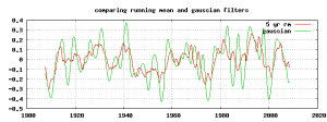
It can be noted that the peaks and troughs in the running mean are absolutely wrong. When the raw data has a peak the running mean produces a trough. This is clearly undesirable.

The data is “smoother” than it was but its sense is perverted. This highlights the difference between simply “smoothing” data and applying appropriately chosen low-pass filter. The two are not the same but the terms are often thought to be synonymous.

Some other filters, such as the gaussian, are much more well behaved, however a gaussian response is never zero, so there is always some leakage of what we would like to remove. That is often acceptable but sometimes not ideal.

Comparing frequency of gaussian and running mean
figure 2 showing the magnitude of the frequency response. However, it should be noted that the sign of every other lobe of running mean is negative in sign, actually inverting the data.

Below is a comparison of two filters ( running mean and gaussian ) applied to some synthetic climate-like data generated from random numbers. Click to see the full extent of the graph.

rm_gauss_AR1
Figure 3. Showing artefacts introduced by simple running mean filter.

As well as the inversion defect, which is again found here around 1970, some of the peaks get bent sideways into an asymmetric form. In particular, this aberration can be noted around 1958 and 1981. In comparing two datasets in order to attribute causation or measure response times of events, this could be very disruptive and lead to totally false conclusions.


Triple running mean filters

Another solution is to improve the running mean’s frequency response.

The sinc function has the maximum of the troublesome negative lobe at πx=tan(πx). Solving this gives πx=1.4303 πx=1.3371…..
[Thanks to Peter Mott for pointing out the error.]
However, simply targeting the peak in the lobe does not produce optimal results. Reduced values leave less residual.

Now if a second running mean is passed after the first one with a period shorter by this ratio, it will filter out the the inverted data…. and produce another, smaller, positive lobe.

A similar operation will kill the new lobe and by this stage any residual problems are getting small enough that they are probably no longer a problem.

The triple running mean has the advantage that it has a zero in the frequency response that will totally remove a precise frequency as well letting very little of higher frequencies through. If there is a fixed, known frequency to be eliminated, this can be a better choice than a gaussian filter of similar period.

The two are shown in the plot above and it can be seen that a triple running mean does not invert the peaks as was the case for the simple running mean that is commonly used.

Example.

With monthly data it is often desirable to remove an annual variation. This can be approximated by the 12,8,6 triple RM shown:

12 / 1.3371 = 8.8975
12 / 1.3371 / 1.3371 = 6.712

It can be seen the second stage is pretty accurate but the final one is rather approximate. However, the error is not large in the third stage.


Figure 4. Comparing frequency response of gaussian and triple running mean filters.

A similar operation on daily data would use: 365, 273, 204

365.242 / 1.3371 = 273.29
365.242 / 1.3371 / 1.3371 = 204,39

Another advantage is that the data from r3m filter really is “smooth” since it does not let past some high frequencies that a simple running mean does. If the aim is simply to “smooth” the data, rather than target a specific frequency, a r3m filter with half the nominal width often gives a smoother result without losing as much information, as was shown in figure 1.

This defect in the smoothing can be seen in the example plot. For example, there is a spike near 1986 in the simple running mean. Worst of all this is not even a true spike in the data that is getting through the filter, it is an artefact.

Another example is the official NOAA [2] presentation of sun spot number (SSN) taken from SIDC [3], examined here:

In 2004, Svalgaard et al published a prediction of the cycle 24 peak [4]. That prediction has proved to be remarkably accurate. It would be even more remarkable if SIDC were to apply a “smoothing” filter that did not invert and displace the peak and reduce its value.

Using direct polar field measurements, now available
for four solar cycles, we predict that the approaching solar
cycle 24 (~2011 maximum) will have a peak smoothed
monthly sunspot number of 75 ± 8, making it potentially the
smallest cycle in the last 100 years.

SIDC processing converts a later trough into the peak value of cycle 24. The supposed peak aligns with the lowest monthly value in the last 2.5 years of data. Clearly the processing is doing more than the intended “smoothing”.

The filter used in this case is a running mean with the first and last points having reduced weighting. It is essentially the same and shares the same defects. Apparently the filter applied to SIDC data was introduced by the Zürich observatory at the end of the 19th century when all these calculations had to be done by hand ( and perhaps the defects were less well understood ). The method has been retained to provide consistency with the historical record. This practise is currently under review.

While it may have been a reasonable compromise in 19th century, there seems little reason other than ignorance of problems for using simple running mean “smoothers” in the 21st century.

Conclusion

Referring to a filter as a “smoother” is often a sign that the user is seeking a visual effect and may be unaware that this can fundamentally change the data in unexpected ways.


Wider appreciation of the corruption introduced by using running mean filters would be beneficial in many fields of study.


Refs.

  [1] Plot of sinc function http://mathworld.wolfram.com/SincFunction.html

  [2] NOAA/Space Weather Prediction Center http://www.swpc.noaa.gov/SolarCycle/index.html

  [3] SIDC sunspot data: http://sidc.oma.be/sunspot-data/
SIDC readme: http://sidc.oma.be/html/readme.txt
SIDC applies a 13 point running mean with first and last points weighted 50%. This is a slight improvement on a flat running mean but shares the same tendancy to invert certain features in the data.

  [4] Svalgaard, L.,E. W. Cliver, and Y. Kamide (2005), Sunspot cycle 24: Smallest
cycle in 100 years?, Geophys. Res. Lett., 32, L01104, doi:10.1029/
2004GL021664. http://www.leif.org/research/Cycle%2024%20Smallest%20100%20years.pdf

Appendix

Scripts to automatically effect a triple-running-mean are provided here:

triple running-mean filter

Example of how to effect a triple running mean on Woodfortrees.org :
http://www.woodfortrees.org/plot/rss/from:1980/plot/rss/from:1980/mean:60/plot/rss/from:1980/mean:30/mean:22/mean:17

Example of triple running mean in spread sheet:
https://www.dropbox.com/s/gp34rlw06mcvf6z/R3M.xls

[Update]

The main object of this article was to raise awareness of the strong, unintentional distortions introduced by the ubiquitous running mean “smoother”.

Filter design is a whole field of study in itself, of which even an introduction would be beyond the scope of this short article. However, it was also an aim to suggest some useful replacements for the simple running-average and to provide implementations that can easily be adopted. To that end, a small adjustment has been made to the r3m.sh script provided and another higher quality filter is introduced:

lanczos3 vs 3-pole RM

A script to implement a low-pass Lanczos filter is provided here: https://climategrog.wordpress.com/2013/11/28/lanczos-filter-script/

An equivalent high-pass filter is provided here: https://climategrog.wordpress.com/2013/11/28/lanczos-high-pass-filter/

High-pass filters may be used, for example, to isolate sub-annual variability in order to investigate the presence or absense of a lunar infulence in daily data.

An example is the 66 day filter used in this analysis:

pink ice triplet

The following points arose in discussion of the article.

Vaughan Pratt points out that shortening the window by a factor of 1.2067 (rather than 1.3371 originally suggested in this article) reduces the stop-band leakage. This provides a useful improvement.

Further optimisation can be attained by reducing negative leakage peaks at the cost of accepting slightly more positive leakage. Since the residual negative peaks are still inverting and hence corrupting the data, this will generally be preferable to simply reducing net residuals irrespective of sign.

The asymmetric triple running-mean is shown in the comparison of the frequency responses, along with a Lanczos filter, here:

lanczos3 vs 3-pole RM detail

The Pratt configuration and the asymmetric 3RM result in identical averaging intervals when set to remove the annual cycle from monthly data. Both result in a choice of 8,10 and 12 month windows.

The difference will have an effect when filtering longer periods or higher resolutions, such as daily data.

If this is implemented in a spreadsheet, it should be noted that each average over an even interval will result in a 0.5 month shift in the data since it is not correctly centred. In a triple running-mean this results in 1.5 months shift with respect to the original data.

In this case the 1.3371 formula originally suggested in the article, giving 12,9,7 month averages and producing just one 0.5 month lag, may be preferable.

None of these issues apply if the scripts provided accompanying the article are used, since they all correctly centre the data.

A more technical discussion of cascading running-mean filters to achieve other profiles can be found in this 1992 paper, suggested by Pekka Pirilä and should serve as a starting point for further study of the subject.

Click to access Gaussian%20Smoothing_96.pdf

exponential decay script (relaxation response)

A simple linear relaxation response leads to an exponentially decaying impulse response. The response to any input can be found by convolution with this impulse response. The following script will apply this convolution with an exponential using a supplied time-constant parameter: tau.

Select text below and use copy / paste to get the text and save to a file. There must be NO space before the first line. ie “#!” are the first characters in the file.

Save as exp-decay.awk , or change messages to suit.

On Linux/Unix-like systems it will need to be given executable permissions.

#!/bin/awk -f

# convolution integral with exp decay kernel eg Laplace 1/s solution
# usage : ./exp-decay.awk filename <tau=12> <neutral=0>
# optional neutral value is subtracted from input data before integration
# use  OFMT="%6.4f"
# tau is time-const of decay fn,  3 tau window is -95% level; 4=98% ; 5=99.3%
# spin-up:  dataset shortened by window length at begining
# ensure data is equally spaced and continuous !!
# nov 2012  OFMT="%10.8f"


BEGIN { OFMT="%10.8f"
# ARGV[1]=filename; argv[0] is script name, hence ARGC>=1

  if  ( ARGC <2 ) {print " usage : ./exp-decay.awk filename <tau=12> <neutral=0>" ; err=1; exit err; }
  if  ( ARGC >3 ) {neutral=ARGV[3];ARGV[3]=""} else {neutral=0};
  if  ( ARGC >2 ) {tau=ARGV[2];ARGV[2]=""} else {tau=12};

  if (neutral != 0) { print "# subtracting neutral point  const of = ",neutral}

kw=4*tau;  # exp(-x) is approx %5 at 3 time-const, prefer 98% accuracy


# calculate normalised kernel coeffs. kernel is time reversed as required
  for (tot_wt=j=0;j<=kw;j++) {tot_wt+=kwt[-j]=exp(-j/tau) };
  for (j=0;j<=kw;j++) {kwt[-j]/=tot_wt};

# strip off last .xxx part of file name

  split(ARGV[1],fn,".");
  for (i=1;i<length(fn);i++){   # if multiple dots in name, build back up except last part
    if(i==1)basename=fn[i]
    else basename=basename"."fn[i];
  }
  out_file=basename"-exp_"tau".dat";

  print "# integrating "ARGV[1]" with exponential decay time const of ",tau
  print "# "ARGV[1]" with exponential decay time const of ",tau >out_file;
  ln=-1;
}

($0 !~ /^#/)&&($0 != ""){
  xdata[++ln]=$1;
  ydata[ln]=$2-neutral;

  if (ln>kw)
  {
    sum=0
    for (j=-kw;j<=0;j++) {sum+=(ydata[ ln+j ])*kwt[j]}
    print NR,xdata[ln],sum
    print xdata[ln],sum >> out_file;  # spin-up: full integral relates to end date of kernel
  }
}

END {
  if (err) exit;
  print "#exp decay kernel width = "kw",done"
  if ( neutral !=0) print "#neutral value = "neutral;
  print "#output file = "out_file
#  for (j=-kw;j<=0;j++) print kwt[j];
}