

[EDIT] above image has been updated with Dec 2015 data.
Introduction
The variation in the magnitude of the annual cycle in arctic sea ice area has increased notably since the minimum of 2007. This means that using a unique annual cycle fitted to all the data leaves a strong residual (or “anomaly”) in post-2007 years. This makes it difficult or impossible to visualise how the data has evolved during that period. This leads to the need to develop an adaptive method to evaluate the typical annual cycle, in order to render the inter-annual variations more intelligible.
Before attempting to asses any longer term averages or fit linear “trends” to the data it is also necessary to identify any repetitive variations of a similar time-scale to that of the fitting period, in order to avoid spurious results.
See also: an examination of sub-annual variation
Method
Short-term anomalies: adapting calculations to decadal variability.
Adaptation can be achieved by identifying different periods in the data that have different degrees of variability and calculating the average annual variation for each period.
Details of how the average seasonal profile for each segment was calculated are shown in the appendix.

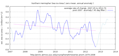
Figure 1. The post-2007 interval. (click to enlarge)
The data was split into separate periods that were identified by their different patterns of variation. For example, the period from 1997 to 2007 has a notably more regular annual cycle (leading to smaller variation in the anomalies). The earlier periods have larger inter-annual variations, similar to those of the most recent segment.
An approximately periodic variation was noted in the data, in the rough form of a rectified sine wave. In order to avoid corrupting the average slope calculations by spanning from a peak to a trough in this pattern, a mathematical sine function was adjusted manually to approximate the period and magnitude shown in the data. It was noted that, despite the break of this pattern in the early 2000’s, the phase of this pattern is maintained until the end of the record and aligns with the post-2007 segement. However, there was a notable drop in level ( about 0.5×10^6 km^2 ). Labels indicate the timing of several notable climate events which may account for some of the deviations from the observed cyclic pattern. These are included for ease of reference without necessarily implying a particular interpretation or causation.

Figure 2. Identifying periods for analysis
The early period (pre-1988) was also separated out since it was derived from a notably different instrument on a satellite with a much longer global coverage. It is mostly from Nimbus 7 mission which was in an orbit with a 6 day global coverage flight path. Somehow this data was processed to produce into a 2 day interval time-series, although documentation of the processing method seems light.
Later data, initially from the US defence meteorology platforms starts in 1988 and had total polar coverage twice per day,producing daily time-series.
In order to maintain the correct relationship between the different segments, the mean value for each segment from the constant term of the harmonic model used to derive the seasonal variations, was retained. The anomaly time-series was reconstructed by adding the deviations from the harmonic model to the mean, for each segment in turn. The calculated anomalies were extended beyond the base period at each end, so as to provide an overlap to determine suitable points for splicing the separate records together. A light low-pass filter was applied to the residual ‘anomalies’ to remove high frequency detail and improve visibility.
The result of this processing can be compared to the anomaly graph provided at the source of this data. The extent of the lines showing mean rates of change indicate the periods of the data used. These were chosen to be an integral number of cycles of the repetitive, circa five year pattern.
Cavalieri et al [2] also report a circa 5 year periodicity:
The 365-day running mean of the daily anomalies suggests a dominant interannual variability of about 5 years

Figure 3. Showing composite adaptive anomaly

Figure 4. Showing Cryosphere Today anomaly derived with single seasonal cycle
Discussion
The average slope for each segment is shown and clearly indicate the decrease in ice area was accelerating from the beginning of the era of the satellite observations until 2007. The derived values suggest this was a roughly parabolic acceleration. This was a cause for legitimate concern around 2007 and there was much speculation as to what this implied for the future development of arctic ice coverage. Many scientists have suggested “ice free” summers by 2013 or shortly thereafter.
The rate of ice loss since 2007 is very close to that of the 1990s but is clearly less pronounced than it was from 1997 to 2007, a segment of the data which in itself shows a clear downward curvature, indicating accelerating ice loss.
Since some studies estimate that much of the ice is now thinner, younger ice of only 1 or 2 years of age, recent conditions should be a more sensitive indicator of change. Clearly the predicted positive feedbacks, run-away melting and catastrophic collapse of Arctic sheet are not in evidence. The marked deceleration since 2007 indicates that either the principal driver of the melting has abated or there is a strongly negative regional feedback operating to counteract it.
The 2013 summer minimum is around 3.58 million km^2. Recent average rate of change is -0.043 million km^2 per year.
While it is pointless to suggest any one set of conditions will be maintained in an ever varying climate system, with the current magnitude of the annual variation and the average rate of change shown in the most recent period, it would take 83 years to reach ice free conditions at the summer minimum.
Some have preferred to redefine “ice free” to mean less than 1 millions km^2 sea ice remaining at the summer minimum. On that basis the “ice free” summer figure reduces to 61 years.
Conclusion
In order to extract and interpret inter-decadal changes in NH sea ice coverage, it is essential to characterise and remove short-term variation. The described adaptive method allows a clearer picture of the post 2007 period to be gained. It shows that what could be interpreted as a parabolic acceleration in the preceding part of the satellite record is no longer continuing and is replaced by a decelerating change in ice area. At the time of this analysis, the current decadal rate of change is about -430,000 km^2 per decade, against an annual average of around 8.7 million and a summer minimum of around 3.6 million km^2.
Whether the recent deceleration will continue or revert to earlier acceleration is beyond current understanding and prediction capabilities. However, it is clear that it would require a radical change for either an ice free ( or an less than one million km^2 ) arctic summer minimum to occur in the coming years.
Unfortunately data of this quality covers a relatively short period of climate history. This means it is difficult to conclude much except that the earlier areal acceleration has changed to a deceleration, with the current rate of decline being about half that of the 1997-2007 period. This is clearly at odds with the suggestion that the region is dominated by a positive feedback.
It is also informative to put this in the context of the lesser, but opposite, tendency of increasing sea ice coverage around Antarctica over the same period.

Figure 5. Showing changes in Arctic and Antarctic sea ice coverage
Figure 3. Showing composite adaptive anomaly
Appendix: approximating the typical seasonal cycle
Spectral analysis of the daily ice area data shows many harmonics of the annual variation, the amplitude generally diminishing with frequency. Such harmonics can be used to reconstruct a good approximation of the asymmetric annual cycle.
Here the typical cycle of seasonal variation for the period was estimated by fitting a constant plus 7 harmonic model to the data ( the 7th being about 52 days ). This is similar to the technique descrobed by Vinnikov et al [1]. The residual difference between the data and this model was then taken as the anomaly for the segment and low-pass filtered to remove 45 day (8th harmonic) and shorter variations.
This reveals an initial recovery from the 2007 minimum and a later drift downwards to a new minimum in 2012. By the time of the annual minimum for 2013, another strong recovery seems to have started.
This repetitive pattern, which was identified in the full record, is used to define trough-to-trough or peak-to-peak periods over which to calculate the average rate of change for each segment of the data. This was done by fitting a linear model to the unfiltered anomaly data ( using a non-linear least squares technique).
Supplementary Information
The fitted average rate of change for the respective periods, in chronological order ( million km^2 per year )
 -0.020

 -0.047

 -0.088

 -0.043
The cosine amplitude, half the total annual variation, of the fundamental of the harmonic model for successive data segments ( million km^2 )
 pre  1988 -4.43

 1988-1997 -4.47

 1997-2007 -4.62

 post 2007 -5.14
Mathematical approximation of repetitive pattern used to determine sampling intervals, shown in figure 2.
cosine period 11.16 years ( 5.58 year repetition )

cosine amplitude 0.75 x 10^6 km^2
Resources
Data source: http://arctic.atmos.uiuc.edu/cryosphere/timeseries.anom.1979-2008
(data downloaded 16th Sept 2013)
A extensive list of official sources both arctic and antarctic sea ice data can be found here:
[1] Vinnikov et al 2002
“Analysis of seasonal cycles in climatic trends with application to satellite observations of sea ice extent”
http://onlinelibrary.wiley.com/doi/10.1029/2001GL014481/pdf
[2] Cavalieri et al 2003
“30-Year satellite record reveals contrasting Arctic and Antarctic decadal sea ice variability”
