
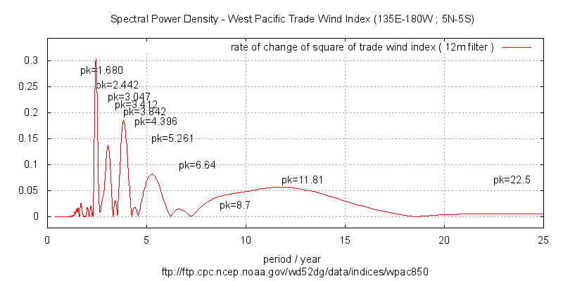
The stem of the letter ‘p’ in the labels indicates the centre of the peak to which it applies. The strongest peak being at 2.442 years.
To evaluate the principal periodicities in the western Pacific Ocean (135E-180W ; 5N-5S), the trade wind index is analysed.
Since many factors in climate are driven by an exchange of energy and constrained by the conservation of energy, the energy of the wind is more relevant in its interaction with other climate variable, the square of wind speed index is used. The trade wind index an “anomaly” time series relative to
1979-1995 average.
The rate of exchange of gases, such as CO2, in and out of the ocean are also found to depend of the square of wind speed [1]
Taking the square makes it dimensionally compatible with other energy terms but is an incorrect estimation since the averaging and the anomaly calculations are done on the wind speed not its square. This remains a better physical variable to analyse than the linear wind speed, in relation to energy transfers in climate.
Since wind speed is strongly influenced by sea surface temperature which itself displays strong autocorrelation, it is preferable to use rate of change for the spectral analysis which removes at least AR(1) autocorrelation. This is required to get accurate spectral analysis.
The spectrum shown is a “chirp-z” frequency analysis of the autocorrelation function. This represents the power density spectrum of the data.
The peaks found from this analysis are:
pk1 0.4444 22.5
pk2 0.0847 11.81
pk3 ~0.11 ~8.7 # significant but unable to resolve peak from 11a
pk4 0.1506 6.64
pk5 0.1901 5.261
pk6 0.2275 4.396 # small
pk7 0.2603 3.842
pk8 0.2931 3.412 # small
pk9 0.328 3.047
pk10 0.4095 2.442
pk11 0.5952 1.680
p7=3.842; p6=4.396; p5=5.261
Interpreting p5,p6,p7 as amplitude modulated (A.M.) side-bands [4]:
26.7368 4.3960 -30.4863
This is somewhat asymmetric. However, allowing a 1% error or perturbation of the central peak, this is a symmetric A.M triplet : ie if pc=4.445 , which seems reasonable:
A.M. side-bands: 28.6583 4.4450 -28.3212
This very close to half the lunar perigee cycle of 8.85 years. Since tidal forces act in both directions, this is likely to produce a component twice that of lunar apsides (perigee) cycle around the equatorial region.
This central frequency of 4.5 years has also been found in the tropical Atlantic Ocean by Dengler et al[2].
Similarly, Clarke et al 2007 [3] details a natural oscillatory period of the equatorial Pacific with a comparable period of 51 months. ( 4.25 years )
pk7=3.842, pk8=3.412, pk9=3.047
Interpreting p7,p8,p9 as A.M. sidebands:
From A.M. sidebands: 30.5658 3.4130 28.4137
Carrier * modulator: 3.3986 * 29.4505
Similarly, accepting the difference between 3.41 and 3.40 as measurement error gives a precise AM triplet corresponding to 3.40 modulated by 29.45 .
It is noted that p7 is used twice here however, the strength of the peak seems sufficient for it to result from contributions from triplets of both its neighbours.
The circa 4.4 year frequency is barely present in the spectrum, indicating nearly 100% modulated by another component of around 28.5 years (sensitivity to error is high on the latter figure, so it may be inaccurate).
The peak tentatively labelled “8.7” is very poorly resolved from the broad spread of energy around 11.8. This means determining the peak is not possible in this plot. However, it quite possible this is twice the previous figure (ie 8.88 years) which is thus also likely to be a manifestation of the lunar perigee cycle of 8.85 years.
There is a possible modulation relationship between pk11, pk10 and pk5.
1.00 + 5.261 year => 1.6806 mod 2.4694 20.16mo mod 29.63mo The latter is close to various values given for the QBO. Conversely, a modulation of a 2y periodicity by 10.8y would also produce peaks 10 and 11:
2.00 mod 10.8 year => 1.6875 mod 2.4545
11.8 and 22.5 are suggestive of Hale / Schwabe solar cycles. They will be a lot more powerful in the time series since longer period components are attenuated in rate of change relative to time series, to a degree proportional to the period.
So the 11.8 year peak would have about the same height as the 2.44 year peak in the time series data.
11.81 is also very close to the sideral period of Jupiter: 11.86 years
The 1.680 peak will have been notably attenuated by the 12m filter so is more significant that is apparent in the graph. As noted above this frequency will result from superposition of 5.26y and the annual cycle.
The data set used here runs from 1981 to 2013, 32 years. So it is likely that the modulation patterns indicating modulation around 30 years is likely to be a result of the windowing function necessary prior to doing the spectral analysis. A Kaiser-Bessel window was used and this is roughly similar in form to a cosine having minima at each end of the data sample. It will have an effect like a 30 year modulation of data. This means that the real spectrum will be simpler that that produced by the analysis with the triplets condensing the total power of the three peaks into a single, more powerful central peak.
The shorter modulations are likely to be physically real.
To get maximum accuracy out from the spectral analysis the very strong annual signal was removed with a low pass filter . This can also be seen to severely attenuated other short periods so this plot will not show the significant content around and below one year.
Data source:
ftp://ftp.cpc.ncep.noaa.gov/wd52dg
References:
[1] Wanninkhof 1992
Relationship Between Wind Speed and Gas Exchange Over the Ocean
[2] Dengler et al 2012
The 4.5-year climate cycle and the mixed layer heat budget in the tropical Atlantic
Current variability associated with the
4.5-year signal exhibits a complex structure
in the upper a equatorial ocean.
Maximum amplitudes of 8cm/s are found on
the equator at 50m depths while the signal nearly
vanishes in the core of the EUC
below. Additionally, the phase distri-
bution indicated a meandering of the
EUC with a period of 4.5-year.
[3] Clarke et al 2007
“Wind Stress Curl and ENSO Discharge/Recharge in the Equatorial Pacific”
http://journals.ametsoc.org/doi/pdf/10.1175/JPO3035.1
The atmosphere responds essentially instantly to the T’ forcing and the curl causes a discharge of WWV during El Niño (T’ > 0) and recharge during La Niña (T’ < 0), so δD'/δt – μT' for some positive constant μ. The two relationships between TЈ and DЈ result in a harmonic oscillator with period 2π/sqrt(μν) Ϸ 51 months.
….
The discharge/recharge oscillator of Jin (1997a,b)
emphasizes the major role of the WWV anomaly [ warm water volume above the thermocline ] and how that leads to a self-sustained coupled ocean–atmosphere oscillation.
[4] Amplitude Modulation Triplets https://climategrog.wordpress.com/2013/09/08/amplitude-modulation-triplets/
